In this blog post we develop a chemistry use case by augmenting classical algorithms for Quantum Monte Carlo with quantum computers. We will explain how to run these quantum-classical hybrid algorithms using Amazon Braket. You can find the code presented in this blog post in an accompanying Jupyter notebook.
Overview
Accurately determining the electronic energies of chemical systems has many applications, including material design and drug discovery. Exact classical methods, such as full configuration interaction (FCI), have memory requirements that scale exponentially with system size. This makes it difficult to simulate many systems of practical interest, such as photovoltaic materials, transition metal-based catalysts, folded proteins, or DNA.
Quantum Monte Carlo (QMC) methods are a family of classical algorithms that circumvent the high memory requirements of FCI methods by performing statistical sampling of the wavefunction. However, the improved scalability of QMC methods comes at the price of reduced accuracy for strongly correlated systems, and an exponential increase in the variance of the energy estimate with system size (known as the ‘sign problem’).
Quantum computation provides new routes to tackling the electronic structure problem. Recently, a series of hybrid quantum-classical QMC methods [1,2,3] have been proposed. These approaches seek to mitigate the aforementioned limitations of classical QMC by augmenting the classical algorithm with a quantum processing unit (QPU). The QMC update steps are still performed on the classical computer. The QPU is used to construct and sample a trial wavefunction that would be intractable to represent on a classical computer. The quantum trial state provides a better approximation to the ground state of the molecule, capturing more of the correlation energy, and thus reducing the bias and variance in QMC calculations.
Quantum Monte Carlo
QMC refers to a class of stochastic methods that sample from the wavefunction, rather than storing and manipulating it. Different QMC variants are better suited for different chemical systems, but all have polynomially scaling memory cost due to their stochastic nature. We focus on auxiliary-field QMC (AFQMC) [4] which represents the target wavefunction as a linear combination of Slater determinant wavefunctions (anti-symmetrized product states of occupied spin-orbitals), referred to as ‘walker states.’ The walker states, |φl〉, can be efficiently manipulated using classical computers. AFQMC exploits this feature to stochastically evolve the walker states in such a way that 1) they remain Slater determinant wavefunctions, and 2) the linear combination of walker states approximates the ground state wavefunction. This process is illustrated below in Figure 1.
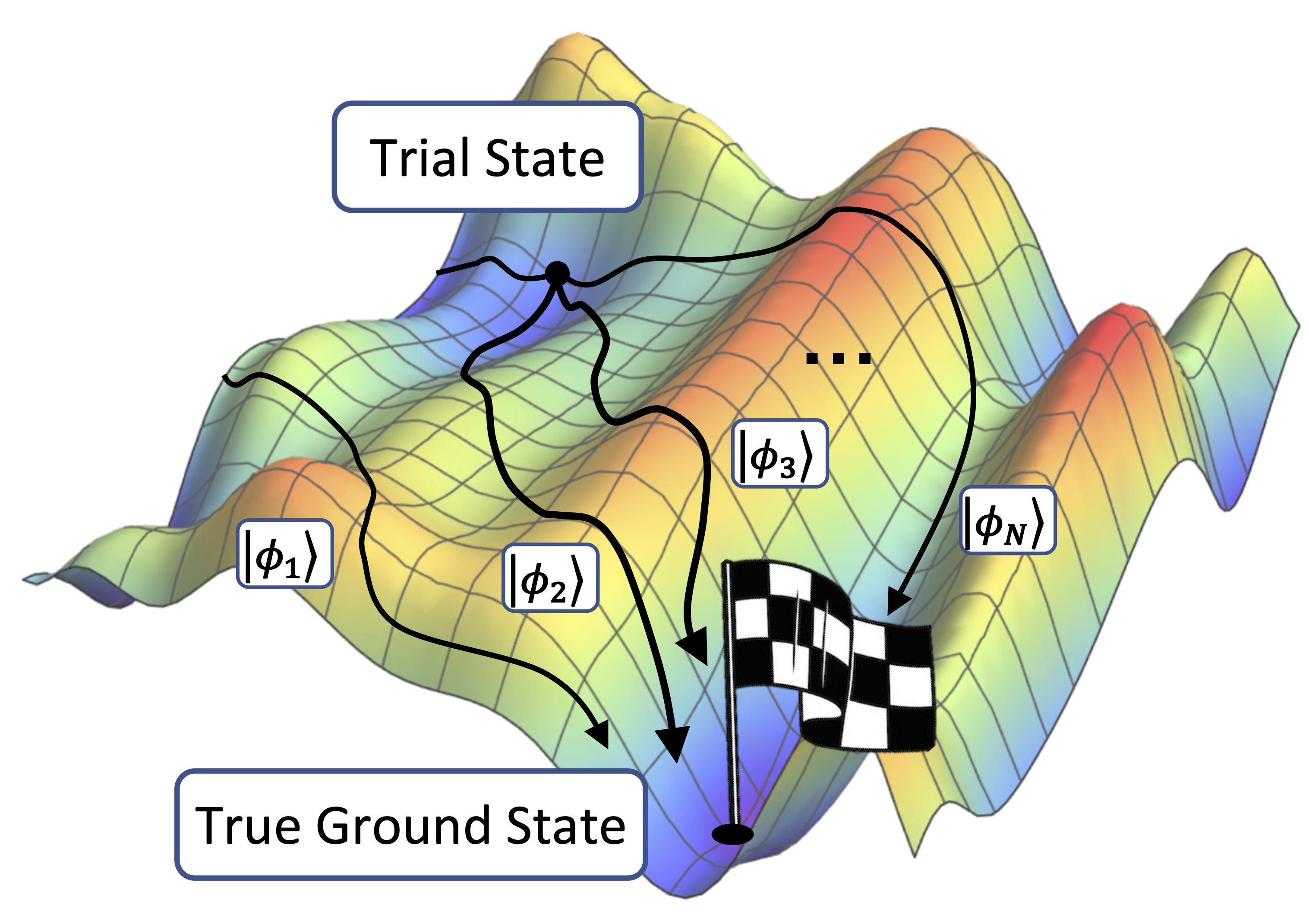
Figure 1. A schematic representation of the AFQMC process, showing walker states, selected via importance sampling, collectively being driven towards the true ground state.
AFQMC is driven by importance sampling from a trial state |ψT〉 , that approximates the true ground state. This is achieved by computing the overlaps 〈φl|ψT〉 and local energies 〈φl|H|ψT〉 between the trial wavefunction and the walker states, at each step of the algorithm. The accuracy of AFQMC depends on the quality of the trial state. Classical computers can only efficiently evaluate these quantities using a restricted class of trial states. Quantum computers, on the other hand, can be used to evaluate the overlaps and local energies with trial states that are hard to prepare on classical computers.
The ease of estimating the overlaps and local energies on QPUs makes AFQMC well suited for a hybrid approach, which we will refer to as quantum-AFQMC (qAFQMC). As shown below in Figure 2, qAFQMC uses the QPU to prepare a trial state that is more accurate than the classical trial state, and measure the overlaps and local energies. The classical computer uses these values to update the walker states according to the standard AFQMC update rules. This process is iterated until the energy converges.
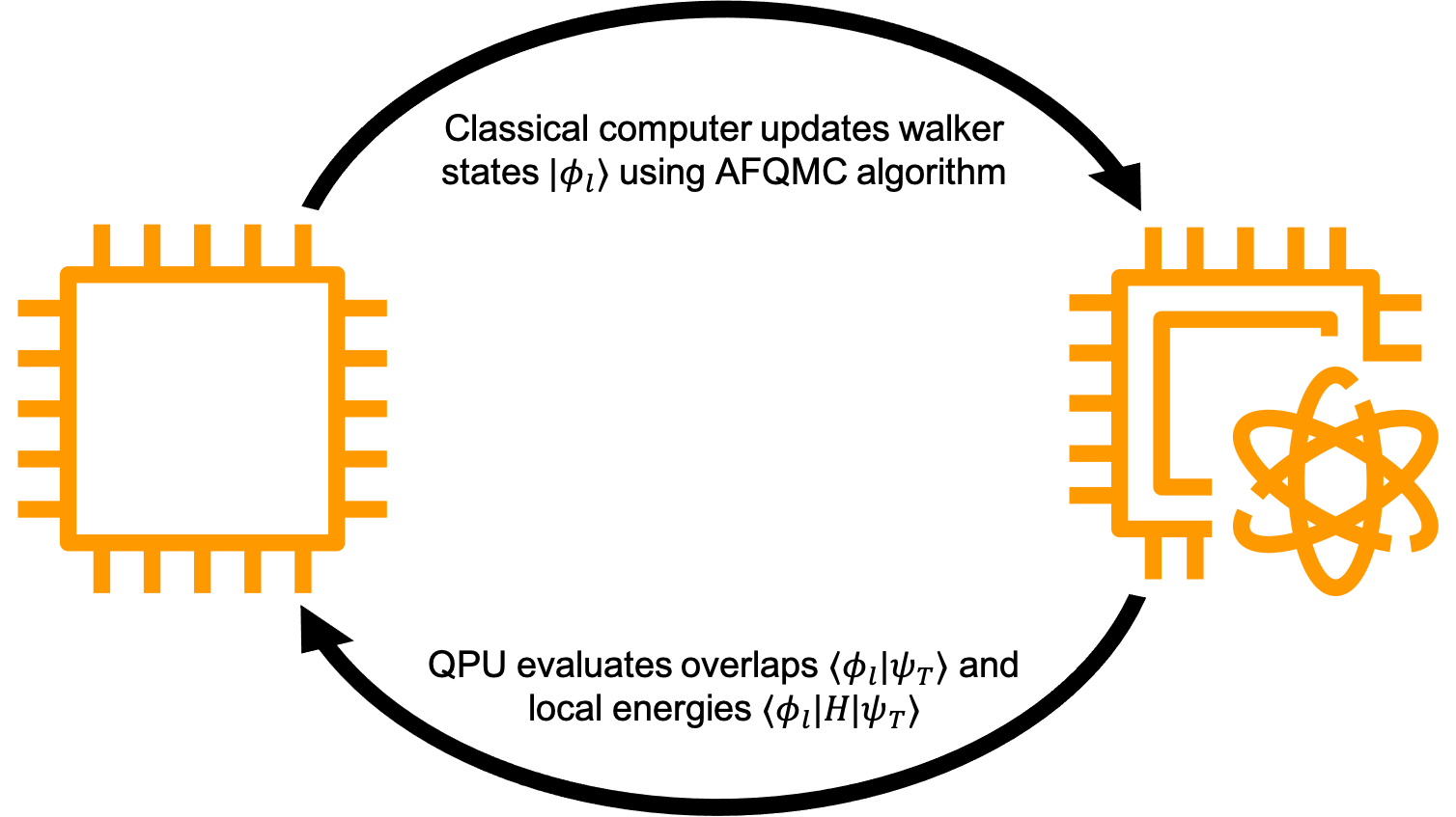
Figure 2. A diagram illustrating the qAFQMC algorithm; the QPU (right) is used to prepare a more accurate trial state and measure the overlaps and local energies. The classical computer (left) uses these values to update the walker states according to the AFQMC update rules.
It is an open research direction to find systems and trial states for which quantum computers are advantageous compared to a purely classical approach. The benefits of qAFQMC for these systems are reduced bias and variance in the energy estimate – at a cost of introducing measurement noise into the algorithm from statistical sampling of the QPU. One can either use the quantum device to assist with both the walker state update and energy evaluation steps of qAFQMC, or just the latter of these steps. Using a quantum device for both steps will increase the accuracy, at the expense of a larger number of quantum circuit evaluations.
qAFQMC has some similarities with the variational quantum eigensolver (VQE), a widely studied algorithm to solve the electronic structure problem on near-term quantum computers. Both the VQE and qAFQMC construct a quantum trial state that approximates the true ground state. In VQE this trial state is optimized in a quantum-classical loop, based on measuring its energy. By contrast, qAFQMC measures the overlaps and energies between the trial state and the walker states, and then performs stochastic evolution of the walker states using these measured values. As such, qAFQMC circumvents the need for the trial state optimization loop at the heart of the VQE.
Setting up the QMC computation
We illustrate qAFQMC by using it to compute the ground state energy of the hydrogen molecule. The code snippet below demonstrates how to instantiate the desired molecule:
# !pip install openfermionpyscf import numpy as np import pennylane as qml from pyscf import gto from afqmc.classical_afqmc import chemistry_preparation, greens_pq, local_energy # Setup. The atom argument provides the geometry of the molecule being studied, for example we # have the hydrogen molecule above, where 0.75 is the bond distance in units of angstrom; molecule = gto.M(atom="H 0. 0. 0.; H 0. 0. 0.75", basis="sto-3g") hf = molecule.RHF() # restricted Hartree-Fock hf.kernel() # compute Hartree-Fock energy and other properties # Define the classical trial state, here we use the Hartree-Fock state as an example. # the dimension of the matrix should be N by N_e, where N is the number of basis functions # and N_e is number of electrons. trial = np.array([[1, 0], [0, 1], [0, 0], [0, 0]]) # Compute chemical properties properties = chemistry_preparation(molecule, hf, trial) # Separate the spin up and spin down channel of the trial state trial_up = trial[::2, ::2] trial_down = trial[1::2, 1::2] # Compute the one particle Green's function G = [greens_pq(trial_up, trial_up), greens_pq(trial_down, trial_down)] # Hartree-Fock energy from the trial state Ehf = local_energy(properties.h1e, properties.eri, G, properties.nuclear_repulsion)Running qAFQMC
The role of the QPU in qAFQMC is to evaluate the overlaps 〈φl|ψT〉 and local energies 〈φl|H|ψT〉. These two quantities are used to compute the total energy of the system, and also drive the update step in the AFQMC algorithm. The quantum circuit shown below in Figure 3 can be used to estimate the overlaps, and can be easily modified to compute the local energies. The circuit uses unitary blocks that prepare the walker state |φl〉 and the trial state |ψT〉. The former can be efficiently implemented using a ‘Givens rotation circuit,’ described in more detail in the accompanying notebook. The latter can be prepared using an ansatz circuit, like those used in the VQE.
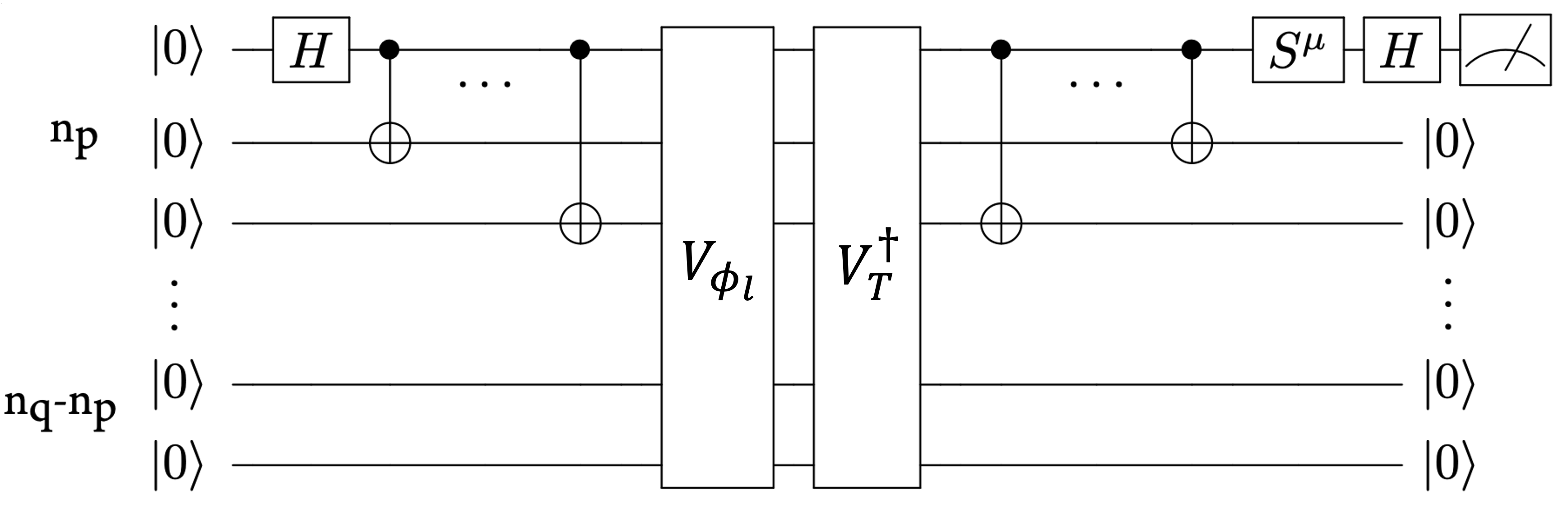
Figure 3. A quantum circuit to evaluate the overlap 〈φl|ψT〉, using unitary circuits that generate the states |ψT〉 and |φl〉 . The parameter μ takes value of 0,1 which determines if the real or imaginary part of the overlap is measured. Here np is the number of electrons, and nq is the number of spin-orbitals. Adapted from Ref [2].
How to parallelize simulators with Amazon Braket
QMC algorithms are naturally parallelizable because each walker state evolves independently. It is straightforward to exploit this parallelization by leveraging the resources available on AWS. In order to rapidly benchmark the algorithm for small system sizes, we opted to use the PennyLane lightning.qubit simulator. This makes it possible to distribute the overlap and local energy calculations across a number of physical cores on a single instance, using the Python multiprocessing module. The code for parallelization of the simulator evaluations across cores is shown below. This function propagates walker states through a number of steps of the qAFQMC algorithm. In this example, we only evaluate the overlaps and local energies on select timesteps (dictated by quantum_evaluations_every_n_steps) and restrict their use to calculating the total energy (as opposed to using them to determine the walker state updates in each step). This reduces the number of circuit evaluations required.
from afqmc.quantum_afqmc import quantum_afqmc dtau = 0.005 num_steps = 1000 num_walkers = 5400 quantum_evaluations_every_n_steps = 10 dev = qml.device("lightning.qubit", wires=4) quantum_energies, energies = quantum_afqmc( num_walkers, num_steps, dtau, quantum_evaluations_every_n_steps, trial, properties, max_pool=36, dev=dev, )The “max_pool” argument controls the number of cores used in the parallelization, and it is used inside the “quantum_afqmc” function shown above.
We can further parallelize the computation using an embedded simulator with Amazon Braket Hybrid Jobs. The Hybrid Jobs feature manages the classical infrastructure required to run hybrid quantum-classical workloads, so researchers can focus solely on developing their algorithm code. With embedded simulators, Amazon Braket supports state-of-the-art simulators from PennyLane, such as the lightning.qubit and lightning.gpu simulators, available directly in the same container as your application code for better runtime performance. In this case, we can use the Hybrid Jobs feature to launch multiple EC2 instances, and distribute the simulator calculation across both the instances and their cores. The code to run qAFQMC as an Amazon Braket hybrid job is shown below:
import time import numpy as np from braket.aws import AwsQuantumJob from braket.jobs.config import InstanceConfig job = AwsQuantumJob.create( device="local:pennylane/lightning.qubit", source_module="afqmc", entry_point="afqmc.run_q_afqmc:run", job_name=f"qaee-afqmc-{int(time.time())}", instance_config=InstanceConfig(instanceType="ml.c5n.18xlarge"), hyperparameters={ "num_walkers": 5400, "num_steps": 1000, "dtau": 0.005, "quantum_evaluations_every_n_steps": 10, "max_pool": 36, }, )In our experiments we distributed the computation across up to ten c5n.18xlarge EC2 instances, each using 36 cores. The resulting improvements to the speed of the qAFQMC algorithm are shown below in Figure 4. Parallelization reduced the runtime from 94 minutes using a single instance to 10 minutes using ten instances. As you only pay for what you use, embedded simulators enable you to parallelize your work across multiple instances – saving time at little to no additional cost. You can refer to our pricing page to learn more about pricing for Hybrid Jobs. Because each walker state evolves independently, each step of AFQMC is an embarrassingly parallelizable problem with near-perfect distribution efficiency.
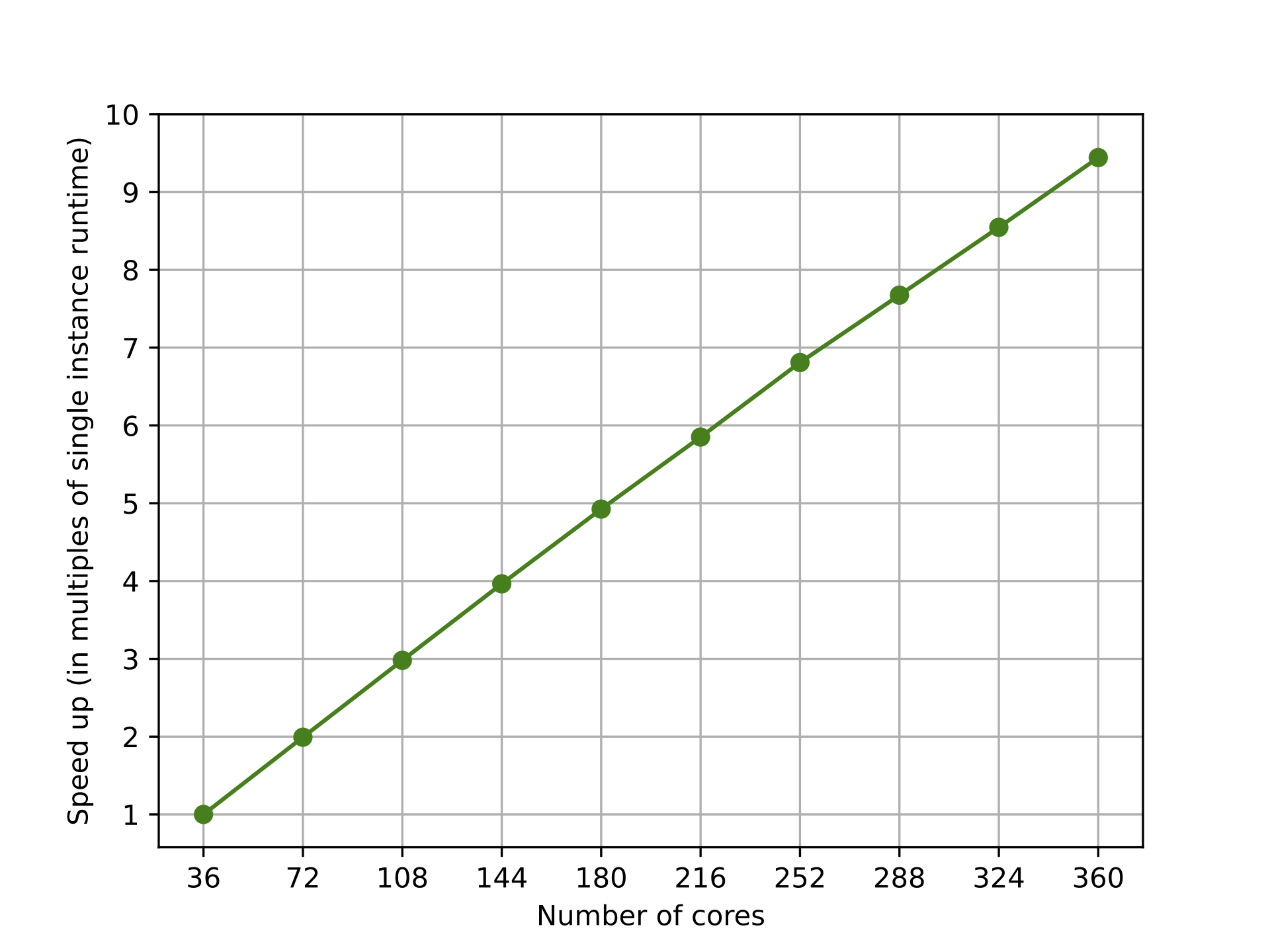
Figure 4. Parallelizing qAFQMC on the PennyLane lightning.qubit simulator across multiple instances (using Amazon Braket Hybrid Jobs) and cores (using the Python multiprocessing module) to reduce the runtime of the algorithm. Parallelization reduced the runtime from 94 minutes using a single instance (36 cores) to 10 minutes using ten instances (360 cores).
Achieving better performance by combining classical and quantum processors
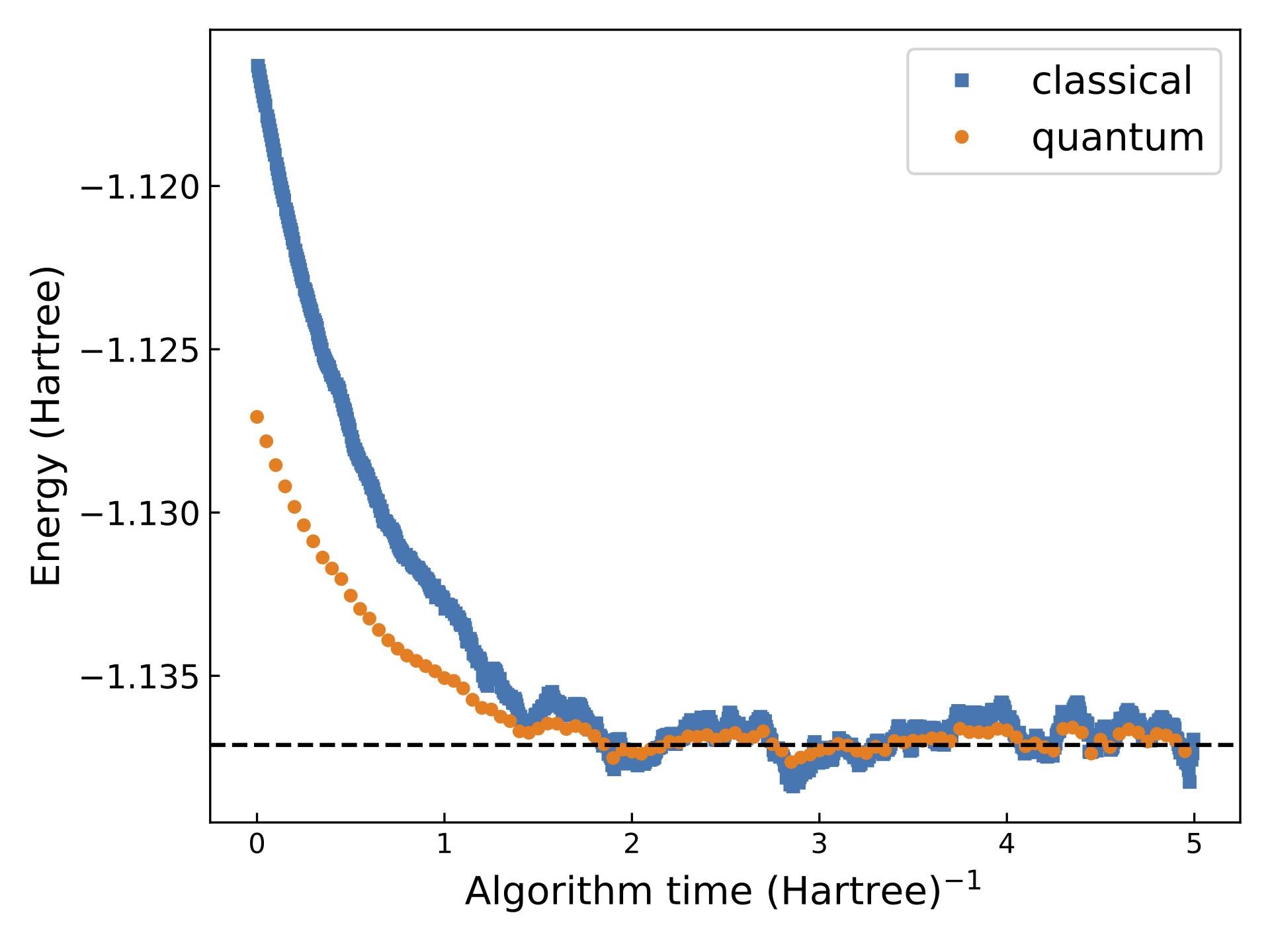
Figure 5. Convergence of classical AFQMC and qAFQMC using 5400 walker states. qAFQMC yielded an energy estimate of −1.136752 Hartree, with a standard deviation of 4.6×10⁻⁴. Classical AFQMC yielded an energy estimate of −1.136358 Hartree, with a standard deviation of 9.4×10⁻⁴. The true energy is −1.137117 Hartree, shown by the dashed line in the figure.
In Figure 5 above, we compare the results of purely classical AFQMC and qAFQMC performed using the PennyLane lightning.qubit simulator (in this example the simulator emulates using a quantum device for energy evaluation at select timesteps). Even for the simple hydrogen molecule, the variance of qAFQMC is smaller by a factor of four than that of its purely classical counterpart, evidenced by the smaller fluctuations in energy upon convergence. For larger, more complex molecules, we also expect to observe a reduction in the bias in the evaluated energy, as a result of using a trial state that better captures the correlation in the molecule.
Conclusion
In this blog post, we have described how quantum computers can augment quantum Monte Carlo algorithms run on classical systems by providing better trial states from which to sample. If you would like to explore and experiment with qAFQMC on Amazon Braket, you can find the code presented in this blog post here. We have illustrated how to modify the code to study new molecules, and optimize the efficiency of the algorithm by using embedded simulators on Amazon Braket. You can learn more about how the Amazon Braket Hybrid Jobs feature enables you to more easily run hybrid quantum-classical workloads here.
References
[1] Huggins, William J., et al. “Unbiasing Fermionic Quantum Monte Carlo with a Quantum Computer.” Nature 603.7901 (2022): 416-420.
[2] Xu, Xiaosi, and Li, Ying. “Quantum-assisted Monte Carlo algorithms for fermions.” arXiv preprint arXiv:2205.14903 (2022).
[3] Zhang, Yukun, et al. “Quantum Computing Quantum Monte Carlo.” arXiv preprint arXiv:2206.10431 (2022).
[4] Zhang, Shiwei. “Auxiliary-Field Quantum Monte Carlo for Correlated Electron Systems.” Emergent Phenomena in Correlated Matter (2013).