Introduction

In recent years, quantum computers have evolved from laboratory experiments available to only a handful of scientists, to research devices that are accessible worldwide through cloud services like Amazon Braket. The impact of cloud access to quantum computers is not limited to laboratory scientists and developers as it allows educators to bring these devices directly into classrooms. AWS partners, like qBraid, are building one-stop quantum computing training platforms on AWS. By utilizing a range of AWS services (e.g., Amazon Elastic Compute Cloud, Amazon Simple Storage Service, or AWS Identity and Access Management) for their platform’s infrastructure, and Amazon Braket for their quantum solutions, qBraid makes it easy for students and working professionals to grow their quantum knowledge.

In this blog post, we present a new qBraid widget, built with Amazon Braket, that introduces two fundamental concepts in quantum computing, the Bloch sphere and the Bernoulli line. The widget comes pre-installed in the home directories of new qBraid accounts. Users are able to perform simulated experiments by manipulating the module’s parameters, observe the system behavior and measurement outcomes on a perfect qubit, then execute the same circuits and measurement on real quantum computers through the Amazon Braket service.

The Bloch sphere is often used in introductory texts to describe the state of a qubit and how one may manipulate this state with single qubit gates. However, bridging the gap between changes in the qubit state and the resulting measurement outcome remains an obstacle for many. Here we will connect these concepts by taking a probability first approach, starting with the Bernoulli line and concluding with measurements results of single qubit states depicted on the Bloch sphere.

The Bernoulli Line

We begin by introducing Bernoulli trials and the Bernoulli line. In a Bernoulli trial, there are two probabilistic outcomes, 0 and 1, e.g., the outcomes of a biased coin. The chances of a obtaining a given result in each trial is determined by the Bernoulli probability parameter, p, represented as a blue dot in Figure 1. If the probability parameter is halfway along the line between the endpoints marked |0> and |1>, then the outcomes occur with equal probability. As the geometrical point (blue dot) moves towards one end or the other of the line (up or down the z-axis) the outcomes are biased towards the corresponding pole. That is, we observe outcome 1 with a higher probability as the blue dot approaches the bottom of the line and observe more 0 outcomes as the dot approaches the top of the sphere.

The correspondence between the geometrical point and the Bernoulli probability parameter, p, is such that is the probability of obtaining outcome 0. The number line for parameter p can be seen as going from p = 0 at the bottom of the line in Figure 1 to at the top. Note this definition of differs from other sources where this parameter corresponds to outcome 1 but is consistent with quantum information conventions.

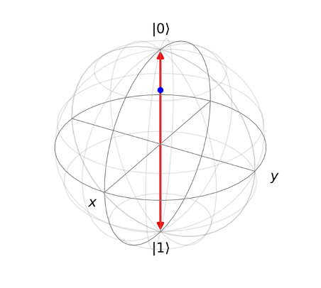
Figure 1: The Bernoulli line is drawn in red spanning from |0⟩ and |1⟩. We use a blue marker to indicate the probability parameter p. Here it is 80% of the distance from the bottom to the top and corresponds to probability, p=0.8, of getting outcome 0.

We can perform a simple Bernoulli trial with Amazon Braket. Consider a Bernoulli trial with p=0.8 that is repeated 1000 times. In Amazon Braket terms, this is a task (a request to a device) consisting of 1000 shots (each shot is a single circuit execution and measurement). The quantum task can be written using the noisy simulation capabilities of the density matrix simulator. The code snippet below uses the local simulator of the Amazon Braket SDK to carry out the Bernoulli trial with p=0.8.

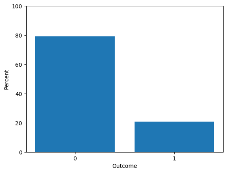
Figure 2: The outcome from 1000 Bernoulli trials with p=0.8 is shown in the bar graph.

The outcomes of repeated trials with the same probability parameter are shown in Figure 2. Notice that the majority of results or “measurements” are 0 as expected because p>0.5.

The Bloch Sphere

Now let us connect our discussion about a point on the Bernoulli line to a one-qubit state, on the Bloch sphere, see Figure 3. In practice, |Ψ> can be created using a quantum circuit. Assuming we initialize |Ψ> = |0> (i.e., with the state vector pointing up along the Z-axis), a single-qubit gate can be visualized as a rotation of |Ψ> on the Bloch sphere. These rotations affect the measurement outcome ratios i.e., number of 0 and 1 outcomes observed. Thus, applying different single-qubit gates has the same effect as changing the Bernoulli probability parameter, p, in the previous experiment.

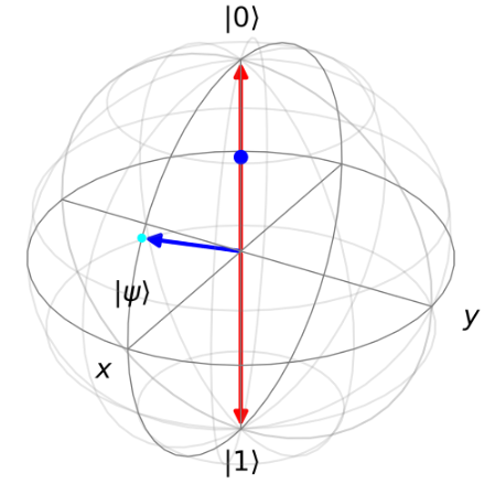
Figure 3: Qubit state vectors, |ψ⟩, generalize the probability parameter of the Bernoulli task. They can be anywhere within the Bloch sphere and must reside on the surface (if the state is pure). The Bernoulli line (red) still determines the outcomes of the shots. The projection of the quantum state onto the Bernoulli line determines the location of the geometrical blue dot which represents the Bernoulli probability parameter, p.

Using Amazon Braket, we can perform the quantum analog of the Bernoulli trial using a parameterized R_y(θ) gate. In the code below, we’ve translated the Bernoulli probability parameter, p, to a quantum gate parameter, θ. Notice that we observe the same behavior with outcome 0 being the dominant outcome.

Rotations about the measurement axis do not affect the projection of the state onto the axis. This is illustrated in the next figure where all states in the animation will generate the same state. This can be seen by observing that the angle in rz(0,np.random.rand()*2*np.pi) has no effect on the plot of the outcomes.

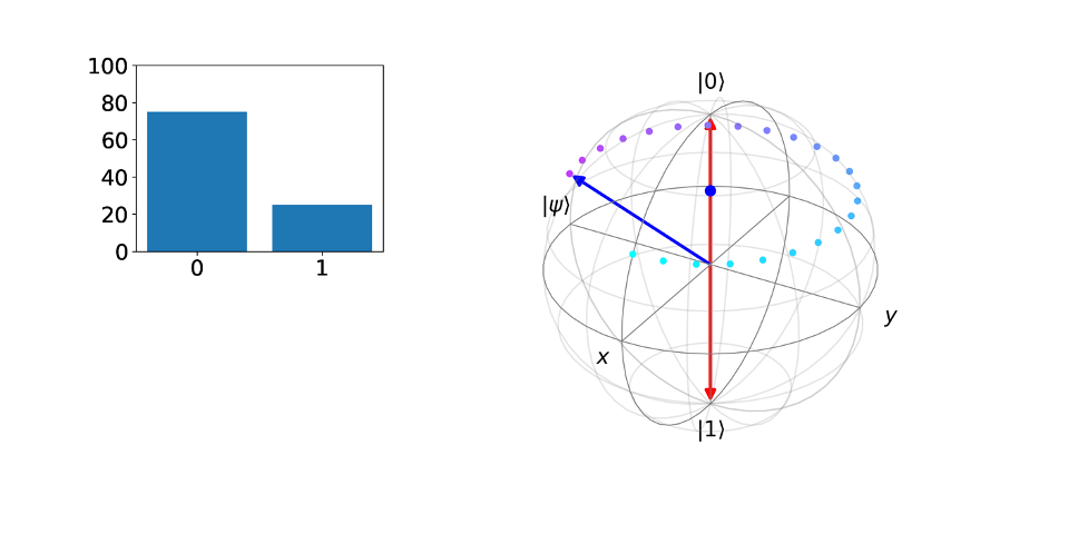
Figure 4: Rotations about the Z axis do not affect the probability parameter since the projection onto the axis is the same of all states depicted in the figure.

Finally, we consider alternatives to measurements in the Z direction, i.e., we will not choose the Bernoulli line to be along the Z direction. Let’s measure in the X direction instead. This is achieved by appending a Hadamard gate to the end of our circuit before performing a standard Z measurement allowing us to observe the projection of |Ψ> onto a Bernoulli line on the X-axis depicted by the green square marker along the X-axis of the next figure. The green geometrical marker corresponds to a Bernoulli probability parameter for outcome +X.

Figure 5: We have plotted the same state |ψ⟩ but now we also show the projection on the X-axis. The green probability parameter indicates the Bernoulli parameter along the X-direction.

When measuring the state in alternative directions, we can keep the same state preparation circuit that initially created |Ψ>. Then we can change the observable being measured using results types. The following code snippet generates the same state as before but also includes a measurement circuit to rotate the Bernoulli line and the output generate the lower green bar graph shown in the previous figure.

Next steps

On qBraid, the widgets provided will allow you to independently vary the parameters of the quantum state and of the measurement axis. Additionally, sequences of one-qubit gates can be visualized with the Bloch sphere. The widget introduced in this blog is available in the qBraid platform along with an extensive set of quantum computing courses to help you get started on your quantum journey. qBraid makes it incredibly simple for anyone to start learning quantum computing: an account is free. Once you login, you will have access to an entire platform with the Jupyter notebook features you expect, a suite of preinstalled quantum software packages in isolated python environments, and access to a range of quantum hardware providers.

With interactive visualizations of qBraid and quantum technology tools of Amazon Braket, this gives a new way of learning about quantum physics and computing. From the Bernoulli line to the Bloch sphere, begin your quantum journey today.